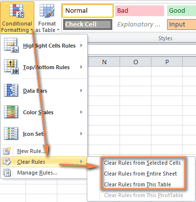
I am trying to take the conditional formatting rules from one cell and apply them to another cell that is formatted differently as standard. Judging by this set of examples of.PasteSpecial enums there isn't one that does the exact job - xlPasteAllMergingConditionalFormats looks like it comes close but I don't actually want to paste anything from one cell to another. Before you clear conditional formats, you may want to verify where they are currently applied. Free outlook for mac. Excel provides a convenient shortcut to select all cells To remove conditional formatting from the table only, select the score values and choose 'Clear rules from selected cells' from the 'Clear Rules' item.

The tutorial explains the basics of Excel conditional formatting feature. You will learn how to create different formatting rules, how to do conditional formatting based on another cell, how to edit and copy your formatting rules in Excel 2007, 2010 2013, and 2016. Using youtube-dl on mac for dummies youtube.

Excel conditional formatting is a really powerful feature when it comes to applying different formats to data that meets certain conditions. It can help you highlight the most important information in your spreadsheets and identify variances of cells' values with a quick glance. At the same time, Conditional Formatting is often deemed as one of the most intricate and obscure Excel functions, especially by beginners. If you feel intimidated by this feature too, please don't! In fact, conditional formatting in Excel is very straightforward and easy to use, and you will make sure of this in just 5 minutes when you have finished reading this short tutorial. • • • • • • • The basics of Excel conditional formatting The same as usual cell formats, you use conditional formatting in Excel to format your data in different ways by changing cells' fill color, font color and border styles. The difference is that conditional formatting is more flexible, it allows you to format only the data that meets certain criteria, or conditions.

You can apply conditional formatting to one or several cells, rows, columns or the entire table based on the cell contents or based on another cell's value. You do this by creating rules (conditions) where you define when and how the selected cells should be formatted. Where is conditional formatting in Excel? For a start, let's see where you can find the conditional formatting feature in different Excel versions.

And the good news is that in all modern versions of Excel, conditional formatting resides in the same location, on the Home tab > Styles group. Conditional formatting in Excel 2007 Conditional formatting in Excel 2010 Conditional formatting in Excel 2013 and Excel 2016 Now that you know where the conditional formatting feature is located in Excel, let's move on and see what format options you have and how you can create your own rules.

How to create Excel conditional formatting rules To truly leverage the capabilities of conditional format in Excel, you have to learn how to create various rule types. This will help you make sense of whatever project you are currently working on.

Conditional formatting rules in Excel define 2 key things: • What cells the conditional formatting should be applied to, and • Which conditions should be met. I will show you how to apply conditional formatting in Excel 2010 because this seems to be the most popular version these days. However, the options are essentially the same in Excel 2007, 2013 and 2016, so you won't have any problems with following no matter which version is installed on your computer.

• In your Excel spreadsheet, select the cells you want to format. For this example, I've created a small table listing the monthly crude oil prices. What we want is to highlight every drop in price, i.e. All cells with negative numbers in the Change column, so we select the cells C2:C9. • Go to the Home tab > Styles group and click Conditional Formatting. You will see a number of different formatting rules, including,. • Since we need to apply conditional formatting only to the numbers less than 0, we choose Highlight Cells Rules > Less Than.

Of course, you can go ahead with any other rule type that is more appropriate for your data, such as: • Format values greater than, less than or equal to • Highlight text containing specified words or characters • Highlight duplicates • Format specific dates • Enter the value in box in the right-hand part of the window under ' Format cells that are LESS THAN', in our case we type 0. As soon as you have entered the value, Microsoft Excel will highlight the cells in the selected range that meet your condition.