1/27/11 7:35 pm MacMost: Numbers & Excel for Mac transferability I use Numbers at home and know my way around it pretty well but have to use Excel for Mac (08) at work. In Excel, I can’t figure out how to create a column with a total at the bottom that I could continue to add data to without leaving a bunch of empty cells. In Numbers I would add a footer row and sum the column. Can I do this in Excel? Or if I create the spreadsheet in Numbers and then open it in Excel will that still work?

Basically I have figures in one column because I need to total them both in categories and then all together but I will be adding figures to this on an ongoing basis. Can’t figure out how to do this on Excel!

Convert your data into Excel Table to get total for your column; How to sum a column in Excel with one click. There is one really fast option. Just click on the letter of the column with the numbers you want to sum and look at the Excel Status bar to see the total of the selected cells. By default, Excel uses the A1 reference style, which refers to columns as letters (A through IV, for a total of 256 columns), and refers to rows as numbers (1 through 65,536). These letters and numbers are called row and column headings. To refer to a cell, type the column letter followed by the row number.

How to get PCSX2 ( PS 2 ) emulator running on Mac OSX. I can only confirm that it does work on 10.8+. It may work on older versions but i have no way of test. The Mac port of PCSX2 requires a few extra bits of software in order to get things running, all of which are free and easily available. While it is possible to dump your own BIOS, you’ll need to execute custom code on the console in order to do so. This will require your PS 2 to be “chipped”, a process. PS 2 Emulator for Mac OS X. PCSX2 is a free and open-source PlayStation 2 emulator for Windows, Linux and macOS that supports a wide range of PlayStation 2 video games with a high level of compatibility and functionality. Look no further then PCSX2, a full blown PS 2 emulator for Mac OS X that works surprisingly well. I say surprising because it seems development work is a little infrequent and there are some features left to be desired, but it certainly works and the frame rate is pretty high on my MacBook. Finally, I can play. Category: Mac. Number of Subcategories: 1. Q1 2018 progress report. The PCSX2 team's statement regarding the 'DamonPS2' emulator.

Any help would be much appreciated!

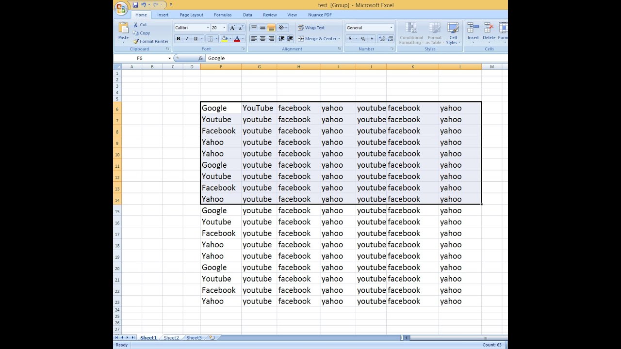
By When sorting your Excel tables and worksheets in Office 2011 for Mac, you’re likely to use ascending and descending sort orders most often. The quick way to sort a table or data range is to select a cell in the column you want to sort. Then go to the Ribbon’s Data tab, find the Sort and Filter group, and click Sort. The first time you click this button, the sort is lowest to highest or alphabetical. Click the button again to sort highest to lowest or reverse alphabetically. Don’t click the column letter before sorting. If you do, the sort will be applied only to the contents of the column, not the entire table or data range.

After 27 years, Microsoft changed the name of this feature from AutoFilter to just Filter? R.I.P., AutoFilter. The Filter feature places a button to the right of each cell in the header row of a table or data range. Filter is turned on by default when you make a table, and you can see these buttons in the header row of a table. You can toggle Filter on or off by pressing Command-Shift-F. When you click the Filter button in a column header, the Filter dialog displays. The column header label is the title of the dialog.

Filter lets you sort and filter. Sorting data in Excel tables The upper portion of the Filter dialog is for sorting: • Ascending: Click this button to sort the column from lowest to highest or alphabetically.

• Descending: Click this button to sort the column from highest to lowest, or reverse alphabetically. • By Color: If you have applied color formats to a table, you can use this pop-up menu to sort by cell color or font color. Filtering data in Excel tables Beneath the Sort functionality is the Filter section of the Filter dialog.

Usually, you know what you’re looking for in a column, so the first thing to do is either type what you want in the search filter or choose it from the Choose One pop-up menu and form field. Starting at the top of the Filter options you can choose: • By Color: Show records in your column that match the cell color, font color, or cell icon. If you haven’t applied colors or conditional formatting, this pop-up menu is inactive. • Choose One: Select a criterion from this pop-up menu.

Then, in the pop-up menu to the right, you can select a record from the column that matches the set of conditions. • Check boxes: You can select and deselect these boxes to display only rows that match the selected items. • Clear Filter button: Removes all criteria from the entire Filter dialog so that no filter or sorting is performed.